Continuing on with my “slight?” obsession with colours… I love colours in “Material Colour Palette”. There various website that will lets you grab the colours by clicking, such as this one, but I just wanted to have little handy cheet sheet for myself, so I’ve decided I’ll do that using R & my favourite ggplot2.
Getting colours out of image using package “imager”
After quick search, I came across image with all the material colour, so first things I’ve tried is to get colours out of image using imager.
## Load up packages we'll use
library(tidyverse)
library(imager)
library(patchwork)

im <- load.image("https://www.materialui.co/img/material-colors-thumb.png")
#plot(im)

## Convert Image to Data Frame with HSV value
im_hsv <-im %>% RGBtoHSV() %>%
  as.data.frame(wide="c") %>%
  rename(h=c.1, s=c.2, v=c.3)

## Convert Image to Data Frame with RGB value
im_rgb <- im %>%
  as.data.frame(wide="c") %>%
  rename(red=c.1,green=c.2,blue=c.3) %>%
  mutate(hexvalue = rgb(red,green,blue)) ## you can create hexvalue using red, green blue value!

## Might as well conver to grayscale, and get luminance.
## I;ll use luminance value to decide if I'll put black text vs white text later.
im_grayscale <- im %>% grayscale() %>%
  as.data.frame() %>%
  rename(luminance=value)

## I want to grab pixel from about middle of each cell
mat_color <- im_rgb %>%
  filter(x %in% as.integer(round(seq(1,19)*(400/19))-10) &
         y %in% as.integer(round(seq(1,11)*(225/11))-10) & y>10) %>%
  left_join(im_hsv) %>%
  left_join(im_grayscale) %>%
  mutate_at(c("x","y"), dense_rank) %>%
  arrange(x,y)


col_group <- c("red","pink","purple","deep purple","indigo","blue","light blue","cyan","teal","green","light green","lime","yellow","amber","orange","deep orange","brown","grey","blue grey")

## Adding extra info to the table
mat_color <- mat_color %>%
  mutate(hue_group=factor(x, labels=col_group, ordered=T),
         shade = factor(y, labels=c(50,seq(100,900, by=100)), ordered=T))

## I could also save this as csv file too... :)
#mat_color %>% write_csv("MaterialColour.csv")
Creating Material Colour Palette Cheat Sheet
Now that I have the colours out of image in data frame, I can do fun stuff, plotting!! I should print this with colour printer, and have it as one of cheat sheet collection.
I’ve used luminance value of each colour to decide if I should place black text or white text over the colour. (I couldn’t figure out if there’s good rules to follow, but seems like luminance does the trick?!)
mat_color %>%
  ggplot(aes(x=hue_group,y=shade)) +  ## I could also use x=x,y=y
  geom_tile(aes(fill=hexvalue),color="white", size=0.1) +  ## i want to have very fine white line around each tiles.
  scale_fill_identity(guide="none") +
  theme_void(base_family="Roboto Condensed") +
  ## print out color hue name and shade
  geom_text(aes(label=paste0(hue_group,"-",shade),
                color=ifelse(luminance>0.5,"#000000","#ffffff")), ## about 48% opacity
            family="Roboto Condensed", size=3, vjust=-2, lineheight=0.8, alpha=0.48) +
  ## print out hesvalue - I'll use this the most, so print it with higher transparency
  geom_text(aes(label=hexvalue,
                color=ifelse(luminance>0.5,"#000000","#ffffff")),  ## about 80% opacity
            family="Roboto Condensed", fontface="bold",vjust=0, alpha=0.8) +
  ## print out RGB & HSV
  geom_text(aes(label=paste0("\n(",round(red*255),",",round(blue*255),",",round(green*255),")\n(",
                             round(h),",",round(s,1),",",round(v,1),")"),
                color=ifelse(luminance>0.5,"#000000","#ffffff")), ## about 67% opacity
            family="Roboto Condensed", size=3, vjust=1, lineheight=0.8, alpha=0.67) +
  scale_color_identity() +
  labs(x="",y="",title="", caption="Material Colour Palettes Hexvalue + RGB + HSV")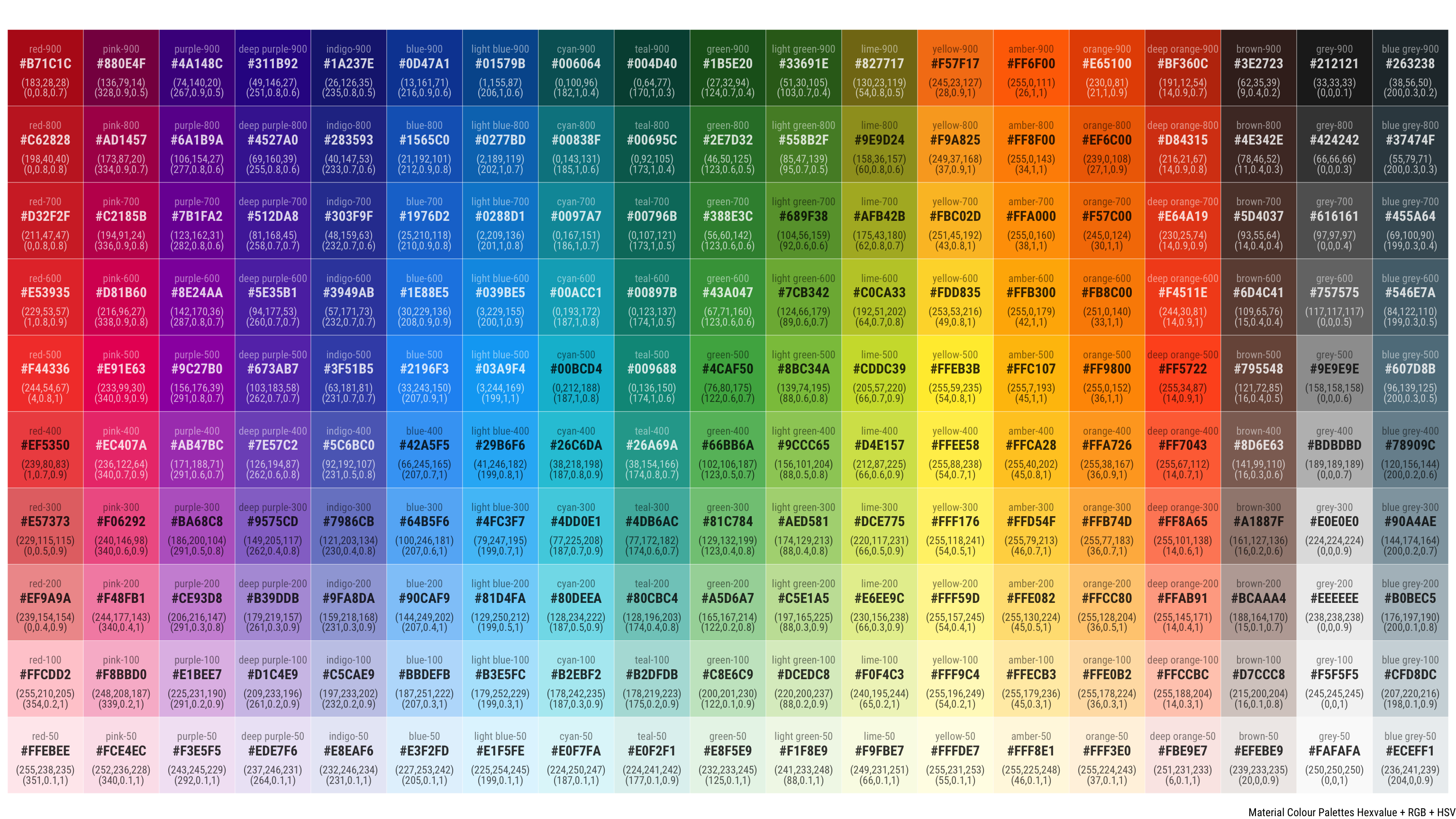
## I can save as PNG file too with below line
#ggsave("MaterialColorCheatSheet.png", width=16, height=9)
More Parrrty Time with Colours…
While plotting colour in rectangular is good…. I thought it’s a lot nicer to plot them as “Colour Wheel”.
# Colour Wheel!
wheel_base <-mat_color %>%
  filter(!hue_group %in% c("brown","grey","blue grey")) %>%  ## exclude brown, grey and blue grey group.
  ggplot(aes(x=x, y=y)) +
  geom_tile(aes(fill=hexvalue), color="white", size=0.1) +
  scale_fill_identity(guide="none") +
  coord_polar() +  ## Converting to polar coordinate does the trick!
  theme_void(base_family="Roboto Condensed") +
  labs(caption="Color Wheel using Material Design Colours")


## Just experimenting with smaller strips on each colour tiles..
wheel_base_w <- wheel_base +
  geom_tile(fill="#ffffffde",height=0.5, aes(width=v*0.5)) +
  labs(caption="If you were to play white text... \nWhich ones can you see better?")

wheel_base_b <- wheel_base +
  geom_tile(fill="#000000de",height=0.5, aes(width=v*0.5)) +
  labs(caption="If you were to play black text... \nWhich ones can you see better?")

## using "patchwork" package I can plot all 3 charts next to each other.
wheel_base + wheel_base_w + wheel_base_b
I wanted to see if I can find pairs of colour that I like by shuffling the colours on smaller strips for fun too.
## Randomize Y
a<-wheel_base +
  geom_tile(aes(fill=hexvalue,y=sample(y)), width=0.5, height=0.5) +
  labs(caption="Randomness within Hue Group")

b<-wheel_base +
  geom_tile(aes(fill=hexvalue,x=sample(x)), width=0.5, height=0.5) +
  labs(caption="Randomness within Same Shade")

## Random Colour Wheel
c<-wheel_base +
  geom_tile(aes(fill=hexvalue,x=sample(x), y=sample(y,replace=T)), width=0.5, height=0.5) +
  labs(caption="Randomness to see if i spot any pairs I like")

a+b+c
Making Some Flowers with Material Colour Palette
## Just for fun, let's just make some flower with material colour palette!
flower1<-mat_color %>%
  arrange(shade,hue_group) %>% mutate(t=row_number()) %>%
  ggplot(aes(x=sqrt(t) * cos(t), y=sqrt(t) * sin(t))) +
  geom_point(aes(color=hexvalue, size=luminance)) +
  #geom_text(aes(label=t), family="Avenir") +
  scale_color_identity() +
  coord_fixed() +
  theme_void(base_family="Roboto Condensed") +
  scale_size_continuous(range=c(3,8), guide="none") +
  labs(caption="Sort by Shade, then Hue Group, Luminance as Size")


## Just for fun, let's just make some flower with material colour palette!
flower2<-mat_color %>%
  arrange(hue_group,shade) %>% mutate(t=row_number()) %>%
  ggplot(aes(x=sqrt(t) * cos(t), y=sqrt(t) * sin(t))) +
  geom_point(aes(color=hexvalue, size=luminance)) +
  scale_color_identity() +
  coord_fixed() +
  theme_void(base_family="Roboto Condensed") +
  scale_size_continuous(range=c(3,8), guide="none") +
  labs(caption="Sort by Hue Group, Then Shade, Luminance as Size")

## ggplot2 has shape 1-25
## 0-15 & 20-24 are NOT filled shape

flower3<-mat_color %>%
  arrange(shade, hue_group) %>% mutate(t=row_number()) %>%
  ggplot(aes(x=sqrt(t) * cos(t), y=sqrt(t) * sin(t))) +
  geom_point(aes(color=hexvalue, shape=ifelse(x<=15,x-1,x+5)), size=3, stroke=1.5) +
  scale_color_identity() +
  coord_fixed() +
  theme_void(base_family="Roboto Condensed") +
  scale_shape_identity() +
  labs(caption="Mapping Hue Groups to Shapes for Fun")

flower1 + flower2 + flower3
One last one for now…
## Final Random Art
mat_color %>%
  ggplot(aes(x=x,y=y)) +
  geom_tile(aes(fill=hexvalue, width=s*10, height=v*10, alpha=luminance)) +
  scale_fill_identity() +
  scale_alpha_continuous(guide="none", range=c(0,0.6)) +
  theme_void() +
  annotate(x=(max(mat_color$x)/2)+0.05,y=(max(mat_color$y)/2)-0.05,
           label="The End",
           geom="text", family="Roboto Condensed", size=22, color="#000000de") +
  annotate(x=max(mat_color$x)/2,y=max(mat_color$y)/2,
           label="The End",
           geom="text", family="Roboto Condensed", size=22, color="#ffffffde") +
  coord_cartesian(xlim=c(0,19), ylim=c(3,7))
Share this post
Twitter
Google+
Facebook
Reddit
LinkedIn
Pinterest
Email